Beyond Equality: Custom Hypotheses with {statim}

Rationale

vignette("htest", package = "statim") covers the t-test example but a rudimentary case: is one mean different from a fixed value, and/or are two means different from each other. Every null hypothesis in that vignette reduces to MU(a) == MU(b) or its one-sample cousin MU(a) == mu.

This vignette is about using weighted, non-zero-threshold claims, not about how state_null() parses them. For the parsing mechanics, see vignette("hypothesis-expressions", package = "statim") — this explains how a coefficient and comparison value are pulled out of an expression like 2 * MU(x) - MU(y) <= 0, and why group order in that expression matters.

Kutner, Nachtsheim, Neter, and Li’s Applied Linear Statistical Models poses a different kind of question throughout its inference chapters: not “are these equal,” but “is a specific weighted combination of these parameters above, below, or at some threshold.” Two things can vary in that question, and they don’t cost the same:

The comparison value. x_by()’s base two-sample path already reads the comparison value straight out of state_null()’s claim. MU(a) - MU(b) <= 3 runs on the ordinary two-sample path — no extra step.
The weights. via("contrast") is the only path in statim that accepts weights other than the implicit +1/-1 split, computing a genuine Welch-Satterthwaite linear contrast (.w) rather than a plain mean difference.

Showcase 2 below is the one place in this vignette where the weights actually depart from ±1. That’s the one place via("contrast") is required — Showcases 1 and 3 stay on the base path.

This vignette isn’t reproducing a specific textbook problem. The book’s own contrast examples mostly involve three or more groups (its ANOVA chapters, already covered by vignette("anova-mod", package = "statim")), while TTEST’s x_by()’s contrast variant is built for exactly two. What it does share with the book is the question type: a weighted, non-zero-threshold claim instead of a plain equality. The three showcases below work that question type through statim, using the same Welch-Satterthwaite machinery the book’s contrast tests are built on.

Setup

Here are the imports for the actual showcase:

box::use(
    statim[
        T_TEST, define_model, prepare, via, state_null, conclude, x_by, MU
    ]
)

ToothGrowth ships with R, so no import step is needed beyond loading it:

data(ToothGrowth)

A look at the data

All three showcases below hinge on the size of the OJ-VC gap, so it’s worth seeing that gap before testing it. Let’s start with stratified summaries (uncover interactions early):

box::use(
    dplyr[mutate, group_by, summarise, keep_when = filter, n],
    forcats[as_factor]
)

ToothGrowth |>
    mutate(dose = as_factor(dose)) |>
    group_by(supp, dose) |>
    summarise(
        n = n(),
        mean = mean(len),
        sd = sd(len),
        
        .groups = "drop"
    )

# A tibble: 6 × 5
  supp  dose      n  mean    sd
  <fct> <fct> <int> <dbl> <dbl>
1 OJ    0.5      10 13.2   4.46
2 OJ    1        10 22.7   3.91
3 OJ    2        10 26.1   2.66
4 VC    0.5      10  7.98  2.75
5 VC    1        10 16.8   2.52
6 VC    2        10 26.1   4.80

Let us check the distribution:

Click here to open

box::use(
    ggplot2[
        ggplot, aes, labs, theme_minimal, theme, element_blank,
        geom_jitter, position_jitter, element_text, element_line,
        element_rect, margin, scale_fill_manual, scale_colour_manual,
        coord_flip, scale_y_continuous
    ],
    ggdist[stat_halfeye, stat_interval, stat_dots],
    patchwork[plot_annotation],
    sysfonts[add_font = font_add_google],
    showtext[showtext_auto],
    ggtext[element_markdown]
)

bg_color = "grey97"
supp_colors = c(OJ = "#B34A44", VC = "#4E7C74")
dodge_width = 0.9

add_font("Lumanosimo", "Lumanosimo")
add_font("Snowburst One", "Snowburst One")
showtext_auto()

subtitle_text = paste0(
    "Distribution, uncertainty, and raw values for tooth growth by dose and supplement ",
    "<br>",
    "**Supplement:** ",
    "<span style='color:#B34A44;'>**Orange Juice (OJ)**</span> | ",
    "<span style='color:#4E7C74;'>**Ascorbic Acid (VC)**</span>"
)

theme_growth = function(subtitle_colour = "grey40") {
    theme_minimal(base_size = 12, base_family = "Lumanosimo") +
        theme(
            legend.position = "none",
            plot.background = element_rect(colour = NA, fill = bg_color),
            plot.title.position = "plot",
            plot.title = element_text(face = "bold", size = 20),
            plot.subtitle = element_markdown(
                colour = subtitle_colour, size = 13, hjust = 0.5,
                family = "Snowburst One",
                lineheight = 1.3,
                margin = margin(t = 6, b = 14)
            ),
            panel.grid = element_blank(),
            panel.grid.major.x = element_line(linewidth = 0.15, colour = "grey80"),
            axis.text.y = element_text(face = "bold"),
            plot.margin = margin(10, 12, 10, 10)
        )
}

Distribution between OJ and VC

ggplot(ToothGrowth, aes(x = supp, y = len, fill = supp, colour = supp)) +
    stat_halfeye(
        alpha = 0.5,
        .width = c(0.5, 0.95),
        point_interval = "median_qi",
        justification = -0.25,
        width = 0.55
    ) +
    geom_jitter(
        position = position_jitter(width = 0.08, height = 0, seed = 1),
        size = 2.2,
        alpha = 0.55,
        show.legend = FALSE
    ) +
    scale_fill_manual(values = supp_colors, guide = "none") +
    scale_colour_manual(values = supp_colors, guide = "none") +
    scale_y_continuous(breaks = seq(0, 35, 10)) +
    coord_flip() +
    labs(
        title = toupper("Same juice, different clouds"),
        subtitle = subtitle_text,
        x = "Supplement",
        y = "Tooth Length"
    ) +
    theme_growth()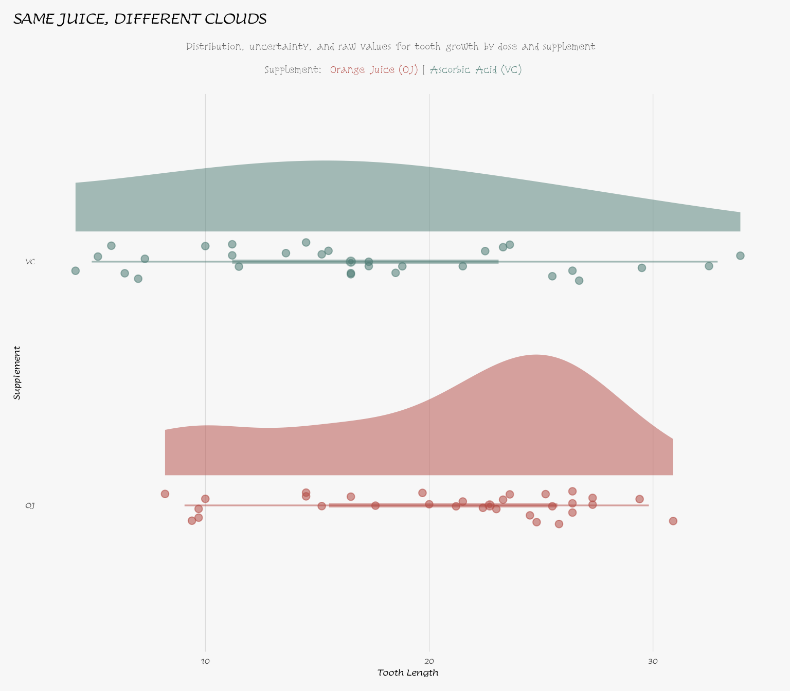

Separated by dose

ggplot(ToothGrowth, aes(x = factor(dose), y = len, fill = supp, colour = supp)) +
    stat_halfeye(
        aes(fill = supp),
        alpha = 0.5,
        position = "dodge",
        .width = c(0.5, 0.95),
        point_interval = "median_qi",
        justification = -0.15,
        width = 0.9
    ) +
    stat_dots(
        aes(fill = supp),
        side = "bottom",
        justification = 1.05,
        binwidth = NA,
        dotsize = 0.8,
        position = "dodge"
    ) +
    scale_fill_manual(values = supp_colors, guide = "none") +
    scale_colour_manual(values = supp_colors, guide = "none") +
    scale_y_continuous(breaks = seq(0, 35, 10)) +
    coord_flip() +
    labs(
        title = toupper("Same juice, different clouds"),
        subtitle = subtitle_text,
        x = "Dose (mg/day)",
        y = "Tooth Length"
    ) +
    theme_growth(subtitle_colour = "#1D2128")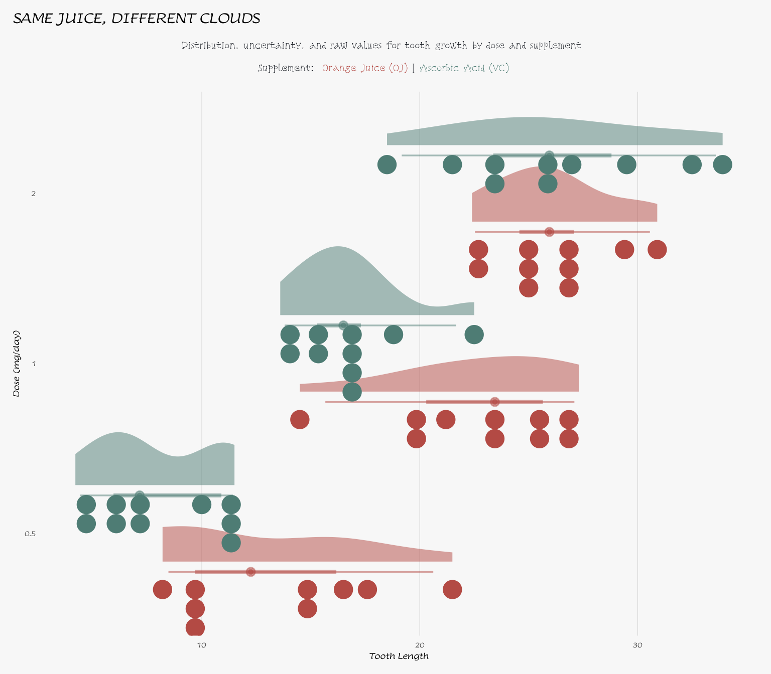

Conditioning on dose

The stratified summary and the plot above agree on something the marginal number hides: the OJ-VC gap is not constant across dose. It runs about 5.25 units at 0.5 mg/day, close to its widest at 5.93 units at 1 mg/day, and collapses to -0.08 units (indistinguishable from zero — at 2 mg/day). Pooling across dose, as a plain two-sample test does, blends a real effect at the two lower doses with a null effect at the highest one. That pooled test puts the marginal gap at 3.70 units and fails to clear a 3-unit bar (p \approx 0.36), a conclusion that dissolves once dose enters the picture.

The three showcases below work within dose == 1, the middle level, where the gap is close to its largest and far from the point where OJ and VC converge. This keeps the worked examples honest about what the data actually support at a fixed dose, rather than testing a pooled average that no individual dose exhibits. A full treatment of the dose effect itself, whether it’s a genuine effect, an interaction with supp, or well-modelled as a factor — is an ANOVA question, not a two-sample one; see vignette("anova-mod", package = "statim").

Showcase 1: Clinically Meaningful Superiority

Question: At 1 mg/day, does OJ outperform VC by more than 3 units (a practically relevant margin)?

H_0: \mu_{\text{OJ}} - \mu_{\text{VC}} \leq 3 \qquad H_1: \mu_{\text{OJ}} - \mu_{\text{VC}} > 3

A plain two-sample test only asks whether the two means differ at all. A textbook question is sharper: is OJ’s advantage over VC big enough to matter, not just big enough to be non-zero. Stating 3 as the comparison value, rather than 0, is what turns this into a genuine contrast rather than a relabeled equality test. The weights are still the default \pm 1 split, so this stays on the base two-sample path (this is valid on stats::t.test(), thus no via("contrast") needed, with an exemption of you wanted to do it).

ToothGrowth |>
    keep_when(dose == 1) |>
    define_model(x_by(len, supp)) |>
    prepare(T_TEST) |>
    state_null(
        MU(len, supp == "OJ") - MU(len, supp == "VC") <= 3
    ) |>
    conclude()


== Model ======================================================================= 

Variable Mapper : x_by 
Args : len | supp 
    x_vars : 1 
    by_vars : 1 

== T-Test ====================================================================== 

-- Summary ---------------------------------------------------------------------

──────────────────────────────────────────
  group  estimate  t_stat    df    p_val  
──────────────────────────────────────────
  supp    5.930    1.993   15.360  0.032  
──────────────────────────────────────────


-- Confidence Interval ---------------------------------------------------------

─────────────────────────────
  group  lower_95  upper_95  
─────────────────────────────
  supp    3.356      Inf     
─────────────────────────────

Interpretation:

At dose == 1, the estimated OJ-VC gap is 5.93, comfortably above the 3-unit bar. t_stat (1.9926) and p_val (0.0322) test that gap against 3, not against zero. At \alpha = 0.05, that’s enough to reject H_0: within this dose, OJ’s advantage isn’t just present, it exceeds 3 units. The one-sided 95% lower bound of 3.3562 makes the same point. The true gap is unlikely to sit at or below the 3-unit bar. Conditioning on dose recovered an effect the marginal test above couldn’t see.

Showcase 2: Weighted Dominance

Question: At 1 mg/day, does twice the mean under OJ still substantially exceed the VC mean?

H_0: 2\cdot\mu_{\text{OJ}} - \mu_{\text{VC}} \leq 0 \qquad H_1: 2\cdot\mu_{\text{OJ}} - \mu_{\text{VC}} > 0

Unlike Showcase 1, the two sides here carry different weights:

2 on one group
1 on the other

So this isn’t a rescaled version of the same null hypothesis. There’s no way to hand base R’s t.test() a coefficient per group; the comparison has to be pre-computed by hand before the call. Here the coefficients live directly in the null hypothesis, and because they aren’t \pm 1, this is the one showcase in this vignette where via("contrast") is required. Drop it and the base path’s claim parser rejects the claim outright, since it only accepts a -1/+1 split.

ToothGrowth |>
    keep_when(dose == 1) |>
    define_model(x_by(len, supp)) |>
    prepare(T_TEST) |>
    state_null(
        # If no coefficient
        # it is hidden and 
        # it contains a coefficient of 1
        2 * MU(len, supp == "OJ") - MU(len, supp == "VC") <= 0
    ) |>
    via("contrast") |>
    conclude()


== Model ======================================================================= 

Variable Mapper : x_by 
Args : len | supp 
    x_vars : 1 
    by_vars : 1 

== T-Test · contrast =========================================================== 

-- Summary ---------------------------------------------------------------------

───────────────────────────────────────────
  group  estimate  t_stat    df    p_val   
───────────────────────────────────────────
  supp    28.630   11.019  10.840  <0.001  
───────────────────────────────────────────


-- Confidence Interval ---------------------------------------------------------

─────────────────────────────
  group  lower_95  upper_95  
─────────────────────────────
  supp    23.958     Inf     
─────────────────────────────

Interpretation:

estimate (28.63) is 2 \cdot \bar{x}_{\text{OJ}} - \bar{x}_{\text{VC}} itself, since .mu is 0 here. p_val is below 0.001, so H_0 is rejected: twice OJ’s mean does not fall short of VC’s, in fact, it’s well above it. The 95% lower bound of 23.9576 says the same thing, since it sits nowhere near 0.

A caveat worth stating plainly: weights of 2, -1 sum to 1, not 0, so this isn’t a contrast in the strict ANOVA sense — it isn’t location-invariant. Shift the origin of the measurement scale and 2 * MU(OJ) - MU(VC) changes value even though the relationship between OJ and VC hasn’t.

Tooth length has a genuine zero (len = 0 means no measurable growth), so the weighting isn’t arbitrary here, but the same expression on a scale without a true zero (Celsius temperature, say) would give a different answer depending on where you happened to put 0. Reach for via("contrast") when you actually need weights other than \pm 1; don’t reach for non-zero-sum weights by default just because the machinery allows it.

Showcase 3: Dynamic Threshold

Question: At 1 mg/day, is the OJ-VC gap at least 20% of the overall (all-dose) average tooth length?

H_0: \mu_{\text{OJ}} - \mu_{\text{VC}} \leq 0.20 \times \bar{x}_{\text{overall}} \qquad H_1: \mu_{\text{OJ}} - \mu_{\text{VC}} > 0.20 \times \bar{x}_{\text{overall}}

Just like Showcase 1, except the comparison value isn’t a number chosen in advance — it’s a data-driven threshold computed from the dataset itself. statim resolves variables from the environment inside state_null(), so you can build flexible, context-aware hypotheses without pre-creating columns or hard-coding numbers. The weights are still \pm 1, so, as in Showcase 1, this stays on the base path where no via("contrast") call is needed.

overall_avg below is computed from the full dataset, all three doses, not the dose == 1 subset under test. It’s meant as an absolute benchmark on the tooth-length scale, not a property of this particular dose.

overall_avg = mean(ToothGrowth$len) # 18.8133

ToothGrowth |>
    keep_when(dose == 1) |>
    define_model(x_by(len, supp)) |>
    prepare(T_TEST) |>
    state_null(
        # An outside variable `overall_avg` is still
        # looked up by `state_null()`
        MU(len, supp == "OJ") - MU(len, supp == "VC") <= 0.20 * overall_avg
    ) |>
    conclude()


== Model ======================================================================= 

Variable Mapper : x_by 
Args : len | supp 
    x_vars : 1 
    by_vars : 1 

== T-Test ====================================================================== 

-- Summary ---------------------------------------------------------------------

──────────────────────────────────────────
  group  estimate  t_stat    df    p_val  
──────────────────────────────────────────
  supp    5.930    1.474   15.360  0.080  
──────────────────────────────────────────


-- Confidence Interval ---------------------------------------------------------

─────────────────────────────
  group  lower_95  upper_95  
─────────────────────────────
  supp    3.356      Inf     
─────────────────────────────

Interpretation:

The estimated OJ-VC gap at dose == 1 is 5.93, the same estimate as Showcase 1. Both showcases test the identical subset and the identical difference, just against different bars. The dynamic threshold (20% of the overall average) is about 3.7627, higher than Showcase 1’s fixed 3-unit bar. t_stat (\approx 1.4739) and p_val (\approx 0.0804) test the gap against this stricter value. At \alpha = 0.05, that’s not quite enough to reject H_0.
Showcase 1 and Showcase 3 report the same confidence interval, (3.3562, \infty). That’s not a “copy-paste” dogma: the interval describes the plausible range for the gap itself, which doesn’t depend on which threshold you’re testing it against. What differs is where each threshold sits relative to that interval. 3 falls below the lower bound (so Showcase 1 rejects), 3.7627 falls above it (so Showcase 3 doesn’t). Same evidence, different bar, different conclusion — which is the entire point of a threshold test.
One footnote: overall_avg is itself estimated from this sample, then treated as fixed once computed. That’s fine for a worked example, but a fully rigorous treatment would need to account for the extra uncertainty in estimating the threshold before testing against it. The interval above reflects sampling uncertainty in the gap only, not in the benchmark.

References

Kutner, M. H., Nachtsheim, C. J., Neter, J., & Li, W. (2004). Applied Linear Statistical Models (5th ed.). McGraw-Hill/Irwin.

Welch, B. L. (1947). The generalization of “Student’s” problem when several different population variances are involved. Biometrika, 34(1-2), 28-35.

Satterthwaite, F. E. (1946). An approximate distribution of estimates of variance components. Biometrics Bulletin, 2(6), 110-114.

Weighted claims, worked through with {statim}

Rationale

Setup

A look at the data

Conditioning on dose

Showcase 1: Clinically Meaningful Superiority

Showcase 2: Weighted Dominance

Showcase 3: Dynamic Threshold

References